Feature Scaling: Intuition behind the math

26 Oct, 2025

I posted this article originally on Notion, sharing here to unify

We’ve all been asked to scale our features to speed up training & steadily decrease our cost. Ever wondered why scaling plays such an important role during model training? Let’s find out!

💭 This blog assumes that you are familiar with the concepts of cost function, gradient descent algorithm

In multivariate linear regression we deal with $n > = 2$ features. These features represent independent variables that have an effect on the dependent variable. Depending on the dataset, each of the features could have a different range of values. For example:

area in sq.ft. $x_{1}$	no. of bedrooms $x_{2}$	price in $ $y$
1800	3	5000
1500	2	4500
2500	5	5600

The cost function for this data with two parameters would look something like this, assuming we use batch gradient descent with batch size of 3

J (θ_{0}, θ_{1}, θ_{2}) = \frac{1}{6} [{(θ_{0} + θ_{1} \cdot 1800 + θ_{2} \cdot 3 - 5000)}^{2} + {(θ_{0} + θ_{1} \cdot 1500 + θ_{2} \cdot 2 - 4500)}^{2} + {(θ_{0} + θ_{1} \cdot 2500 + θ_{2} \cdot 5 - 5600)}^{2}]

If we simplify the above equation, all we have is a quadratic equation of the form

J (θ_{0}, θ_{1}, θ_{2}) = {(θ_{0} + θ_{1} \cdot x_{1} + θ_{2} \cdot x_{2} - y)}^{2}

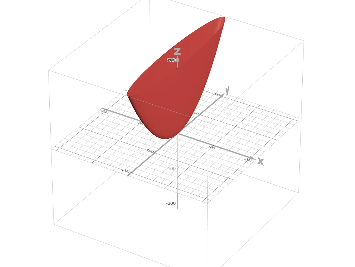
In our dataset, $x_{1}$ is a relatively large value when compared to $x_{2}$ . This makes the shape of the cost function $J$ such that $θ_{1}$ will correspond to the narrow axis and $θ_{2}$ will correspond to the long axis. The function plot will look something like this where $x$ axis represents $θ_{1}$ and y axis represents $θ_{2}$

feature-scaling-1 https://www.desmos.com/3d/wthv10wjki

It’s clear that small changes in $θ_{1}$ have a big impact on $J$ & relatively large changes in $θ_{2}$ have a small impact. The rate of change of $J$ along the direction of each of parameter i.e., gradient components is given by

\frac{\partial J}{\partial θ_{0}} = 2 \cdot (θ_{0} + θ_{1} \cdot x_{1} + θ_{2} \cdot x_{2})

\frac{\partial J}{\partial θ_{1}} = 2 \cdot (θ_{0} + θ_{1} \cdot x_{1} + θ_{2} \cdot x_{2}) \cdot x_{1}

\frac{\partial J}{\partial θ_{2}} = 2 \cdot (θ_{0} + θ_{1} \cdot x_{1} + θ_{2} \cdot x_{2}) \cdot x_{2}

🧠 If $f$ is a multivariate function in $x_{1}$ , $x_{2}$ , a partial derivative of a function w.r.t. $x_{1}$ is just a way of asking how much does $f$ change w.r.t. $x_{1}$ while keeping $x_{2}$ constant.

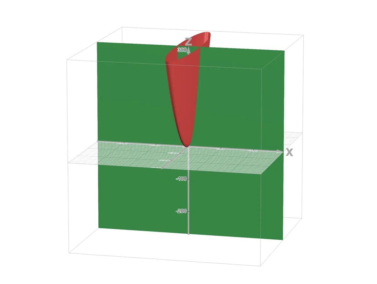
Visually $\frac{\partial J}{\partial θ_{1}}$ looks like this, keeping $θ_{2}$ constant, where the plane cuts the 3-D curve

feature-scaling-2 https://www.desmos.com/3d/yojzjugcw5

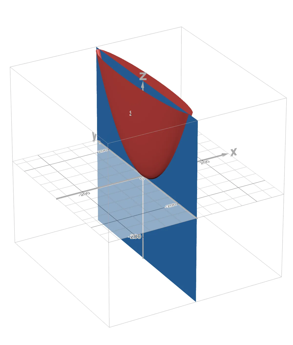
Visually $\frac{\partial J}{\partial θ_{2}}$ looks like this, keeping $θ_{1}$ constant, where the plane cuts the 3-D curve

feature-scaling-3 https://www.desmos.com/3d/kwp9c9zzrm

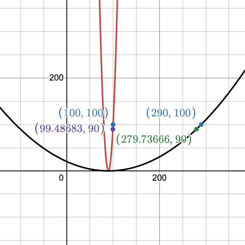
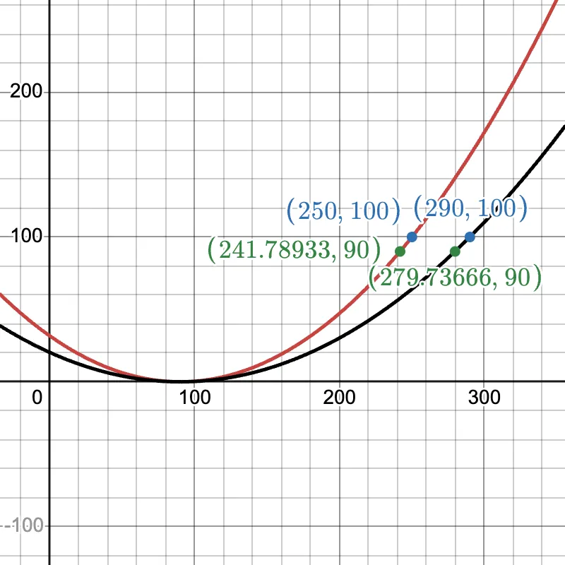
$\frac{\partial J}{\partial θ_{1}}$ is larger as rate of change of $J$ is higher w.r.t. small changes in $θ_{1}$ . Conversly, $\frac{\partial J}{\partial θ_{2}}$ is smaller as rate of change of $J$ is lower w.r.t. small changes in $θ_{2}$ . Visually, by imagining on a 2D axis, we can see that along the narrow axis $θ_{1}$ (red), a small change has a huge impact on $J$ (vertical axis). Along the long axis $θ_{2}$ (black), to change $J$ by the same amount, we need a relatively large change in $θ_{2}$ .

feature-scaling-4 https://www.desmos.com/calculator/i6y8fwmd3m

Let’s plug this information into our parameter update step using gradient descent

θ_{1} = θ_{1} - α \cdot \frac{\partial J}{\partial θ_{1}}

θ_{2} = θ_{2} - α \cdot \frac{\partial J}{\partial θ_{2}}

Faster convergence means having a relatively larger learning rate $α$ . But we run into an issue with his, if $α$ is too large, $θ_{1}$ will overshoot as $\frac{\partial J}{\partial θ_{1}}$ is also large. To counteract this, if we choose a relatively smaller learning rate $α$ , $θ_{2}$ will update very slowly leading to a very slow convergence overall.

That is why we need to scale our features. Scaling helps us choose a good learning rate without having to worry about it’s effect on each of the parameters. This leads to faster & more stable convergence.

feature-scaling-5 https://www.desmos.com/calculator/axjjlwtgyy

With Gratitude
To my family and friends for their support

Sources
Partial derivatives, introduction by Khan Academy